Handling Zman-seq Timestamps

CellDyc was applied to the GBM Monocyte Differentiation dataset (See details here), where temporal information was derived from Zman-seq rather than traditional time-series sampling. Since Zman-seq provides continuous in vivo timestamping, the resulting temporal labeling is highly asynchronous.

Import Packages

import scanpy as sc
import matplotlib.pyplot as plt
import celldyc as cdc

Load the Data

The analysis is based on in-built GBM Monocyte Differentiation dataset.

# Load Zman-seq data
adata = cdc.datasets.mono2tam()
adata

AnnData object with n_obs × n_vars = 3108 × 4407
    obs: 'batch', 'mouse', 'time_assignment', 'cluster_colors', 'n_genes', 'Treatment', 'combined', 'Treatment_cluster'
    uns: 'cluster_colors_colors'
    obsm: 'X_mcg', 'X_pca'
    layers: 'spliced', 'unspliced'

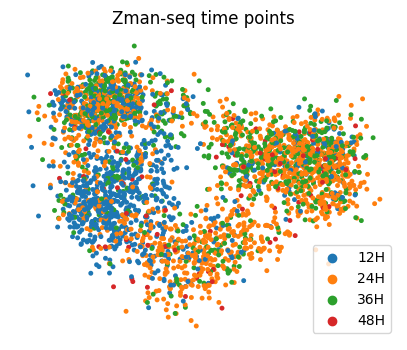
This dataset contains cells from 4 time points and the temporal label is highly asynchronous.

fig, ax = plt.subplots(figsize=(5,4))
ax = sc.pl.embedding(
    adata,
    color=["time_assignment"],  
    basis="mcg",              
    ax=ax,
    title="Zman-seq time points",                 
    legend_loc="lower right",  
    s=50, 
    frameon=False                   
)

Preprocess the Data

adata = cdc.tl.preprocess(adata)

We transform descriptive time point strings into numerical format.

cat_map = {'12H': 12, '24H': 24, '36H': 36, '48H': 48}
adata.obs['numerical_time'] = adata.obs['time_assignment'].map(cat_map).astype('category')

Estimation of Time Representation and Transcriptomic Velocity

We train CellDyc using the recover_dyc function. By default, predicted velocities are stored in adata.layers[‘velocity’], and predicted time values are stored in adata.obs[‘getime’].

cdc.tl.recover_dyc(adata, time_key="numerical_time", time_weight=0.001)

Training with early stop (max_epochs=500, patience=40)
epoch   1:loss=0.926128,trend_loss=0.925350,time_loss=0.778284
epoch  51:loss=0.623676,trend_loss=0.623134,time_loss=0.542161
epoch 101:loss=0.598081,trend_loss=0.597530,time_loss=0.551124
epoch 151:loss=0.577577,trend_loss=0.577017,time_loss=0.560104
Early stopping at epoch 191

AnnData object with n_obs × n_vars = 3108 × 2000
    obs: 'batch', 'mouse', 'time_assignment', 'cluster_colors', 'n_genes', 'Treatment', 'combined', 'Treatment_cluster', 'numerical_time', 'getime'
    var: 'n_cells', 'highly_variable', 'means', 'dispersions', 'dispersions_norm', 'getime_weights'
    uns: 'cluster_colors_colors', 'time_assignment_colors', 'log1p', 'hvg', 'pca', 'neighbors'
    obsm: 'X_mcg', 'X_pca'
    varm: 'PCs'
    layers: 'spliced', 'unspliced', 'velocity'
    obsp: 'distances', 'connectivities'

cdc.pl.getime_violin(adata,"getime","numerical_time",xlabel="Zman-seq time",remove_ticks=False)

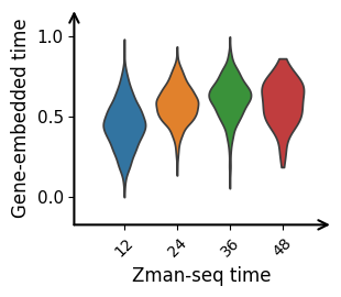
<Axes: xlabel='Zman-seq time', ylabel='Gene-embedded time'>

We then project the velocities onto the metacell graph projection.

cdc.pl.plot_velocity_projection(
    adata, 
    basis="mcg",            
    color='cluster_colors',                        
    legend_loc="right",  
    figsize=(5, 5)          
)

computing velocity graph
finished.

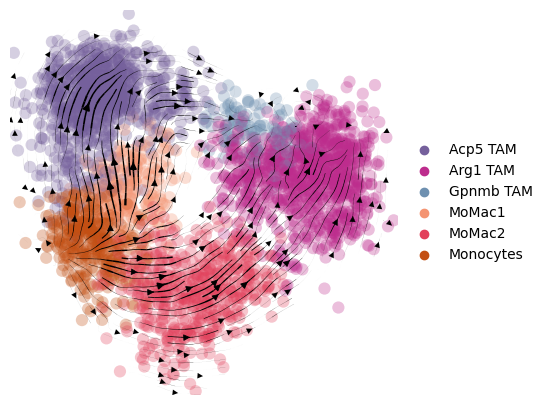
computing velocity embedding
finished.