Recover Masked Time Points in Zebrafish Embryogenesis

CellDyc is applied to the axial-mesoderm lineage of zebrafish embryos (See details here) using data from 12 time points (3.3–12 hours post-fertilization). We first evaluate CellDyc’s performance on the complete dataset containing all 12 time points. Subsequently, we down-sample the dataset to 6 time points for training and apply the trained model back to the full dataset.

Import Packages

import scanpy as sc
import matplotlib.pyplot as plt
import celldyc as cdc

Load the Data

The analysis is based on in-built Zebrafish dataset.

adata = cdc.datasets.zebrafish()
adata

AnnData object with n_obs × n_vars = 2341 × 23974
    obs: 'Stage', 'gt_terminal_states', 'lineages'
    uns: 'Stage_colors', 'gt_terminal_states_colors', 'lineages_colors'
    obsm: 'X_force_directed'

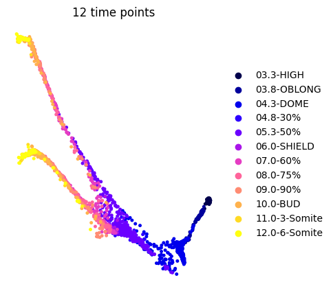
This dataset contains cells from 12 time points.

fig, ax = plt.subplots(figsize=(4,5))
sc.pl.embedding(adata, color="Stage", basis="force_directed", ax=ax,title="12 time points",frameon=False)

Preprocess the Data

adata = cdc.tl.preprocess(adata)
adata

AnnData object with n_obs × n_vars = 2341 × 2000
    obs: 'Stage', 'gt_terminal_states', 'lineages'
    var: 'n_cells', 'highly_variable', 'means', 'dispersions', 'dispersions_norm'
    uns: 'Stage_colors', 'gt_terminal_states_colors', 'lineages_colors', 'log1p', 'hvg', 'pca', 'neighbors'
    obsm: 'X_force_directed', 'X_pca'
    varm: 'PCs'
    obsp: 'distances', 'connectivities'

We transform descriptive time point strings into numerical format.

cat_map = {'03.3-HIGH': 03.3,
           '03.8-OBLONG': 03.8,
           '04.3-DOME': 04.3,
           '04.8-30%':04.8,
           '05.3-50%':05.3,
           '06.0-SHIELD':06.0,
           '07.0-60%':07.0,
           '08.0-75%':08.0,
           '09.0-90%':09.0,
           '10.0-BUD':10.0,
           '11.0-3-Somite':11.0,
           '12.0-6-Somite':12.0}
adata.obs['numerical_time'] = adata.obs['Stage'].map(cat_map).astype('category')

Estimation of Time Representation and Transcriptomic Velocity with all 12 time points

We first train CellDyc using the recover_dyc function. By default, predicted velocities are stored in adata.layers[‘velocity’], and predicted gene-embedded time values are stored in adata.obs[‘getime’].

cdc.tl.recover_dyc(adata, time_key='numerical_time')

Training with early stop (max_epochs=500, patience=40)
epoch   1:loss=0.837947,trend_loss=0.828511,time_loss=0.094358
epoch  51:loss=0.425178,trend_loss=0.424160,time_loss=0.010178
epoch 101:loss=0.385324,trend_loss=0.384423,time_loss=0.009003
epoch 151:loss=0.377774,trend_loss=0.376906,time_loss=0.008671
epoch 201:loss=0.373027,trend_loss=0.372226,time_loss=0.008010
epoch 251:loss=0.352568,trend_loss=0.351829,time_loss=0.007390
Early stopping at epoch 299

AnnData object with n_obs × n_vars = 2341 × 2000
    obs: 'Stage', 'gt_terminal_states', 'lineages', 'numerical_time', 'getime'
    var: 'n_cells', 'highly_variable', 'means', 'dispersions', 'dispersions_norm', 'getime_weights'
    uns: 'Stage_colors', 'gt_terminal_states_colors', 'lineages_colors', 'log1p', 'hvg', 'pca', 'neighbors'
    obsm: 'X_force_directed', 'X_pca'
    varm: 'PCs'
    layers: 'velocity'
    obsp: 'distances', 'connectivities'

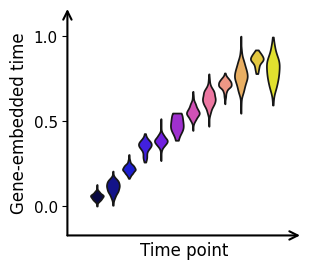
We generated a violin plot of gene-embedded time versus sampling time points, which shows that the learned time respects the actual temporal order.

cdc.pl.getime_violin(adata, 'getime', 'numerical_time',palette='gnuplot2')

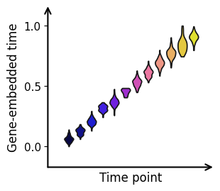
<Axes: xlabel='Time point', ylabel='Gene-embedded time'>

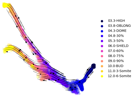
We then project the velocities onto the force-directed embedding.

cdc.pl.plot_velocity_projection(adata,basis='force_directed', color='Stage',figsize=(5,5),legend_loc="right")

computing velocity graph
finished.

computing velocity embedding
finished.

Estimation of Time Representation and Transcriptomic Velocity with 6 time points

adata_ = cdc.datasets.zebrafish()
adata_.obs['numerical_time'] = adata_.obs['Stage'].map(cat_map).astype('category')
sc.pp.filter_genes(adata_, min_cells=10)
sc.pp.normalize_total(adata_, target_sum=1e4)
sc.pp.log1p(adata_)
sc.pp.highly_variable_genes(adata_, n_top_genes=2000)
adata_ = adata_[:, adata_.var.highly_variable].copy()

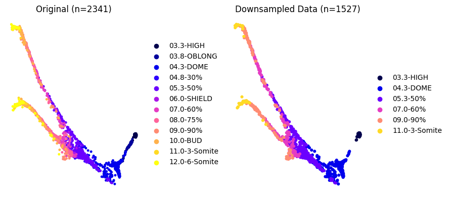
We select subsets at six time points.

keep = ['03.3-HIGH','04.3-DOME','05.3-50%','07.0-60%','09.0-90%','11.0-3-Somite']
adata_subset = adata_[adata_.obs['Stage'].isin(keep)].copy()
fig, axes = plt.subplots(1, 2, figsize=(9,4))
sc.pl.embedding(
    adata, 
    basis='force_directed', 
    color='Stage', 
    ax=axes[0], 
    title=f'Original (n={adata.n_obs})',
    show=False,frameon=False
)
sc.pl.embedding(
    adata_subset, 
    basis='force_directed', 
    color='Stage', 
    ax=axes[1], 
    title=f'Downsampled Data (n={adata_subset.n_obs})',
    show=False,frameon=False
)
plt.tight_layout()
plt.show()

sc.tl.pca(adata_subset, svd_solver='arpack')
sc.pp.neighbors(adata_subset, n_neighbors=30, n_pcs=30)

sc.tl.pca(adata_, svd_solver='arpack')
sc.pp.neighbors(adata_, n_neighbors=30, n_pcs=30)

We then train CellDyc on the downsampled adata_sub and save the trained model to save_path.

cdc.tl.recover_dyc(adata_subset,time_key="numerical_time", save_path='zebrafish.pt')

Training with early stop (max_epochs=500, patience=40)
epoch   1:loss=0.876759,trend_loss=0.862731,time_loss=0.140287
epoch  51:loss=0.313247,trend_loss=0.312212,time_loss=0.010346
epoch 101:loss=0.270490,trend_loss=0.269659,time_loss=0.008309
epoch 151:loss=0.259464,trend_loss=0.258694,time_loss=0.007700
epoch 201:loss=0.244994,trend_loss=0.244285,time_loss=0.007091
epoch 251:loss=0.245265,trend_loss=0.244603,time_loss=0.006618
Early stopping at epoch 256

AnnData object with n_obs × n_vars = 1527 × 2000
    obs: 'Stage', 'gt_terminal_states', 'lineages', 'numerical_time', 'getime'
    var: 'n_cells', 'highly_variable', 'means', 'dispersions', 'dispersions_norm', 'getime_weights'
    uns: 'Stage_colors', 'gt_terminal_states_colors', 'lineages_colors', 'log1p', 'hvg', 'pca', 'neighbors'
    obsm: 'X_force_directed', 'X_pca'
    varm: 'PCs'
    layers: 'velocity'
    obsp: 'distances', 'connectivities'

Next, we apply this saved model to the full 12 time points dataset.

cdc.tl.recover_dyc(adata_, time_key='numerical_time', model_path='zebrafish.pt')

AnnData object with n_obs × n_vars = 2341 × 2000
    obs: 'Stage', 'gt_terminal_states', 'lineages', 'numerical_time', 'getime'
    var: 'n_cells', 'highly_variable', 'means', 'dispersions', 'dispersions_norm', 'getime_weights'
    uns: 'Stage_colors', 'gt_terminal_states_colors', 'lineages_colors', 'log1p', 'hvg', 'pca', 'neighbors'
    obsm: 'X_force_directed', 'X_pca'
    varm: 'PCs'
    layers: 'velocity'
    obsp: 'distances', 'connectivities'

Here, we generate a violin plot of gene-embedded time versus sampling time points, showing that the model—trained on only 6 time points—learns a time representation that respects the actual temporal order across all 12 time points.

cdc.pl.getime_violin(adata_, 'getime', 'numerical_time',palette='gnuplot2')

<Axes: xlabel='Time point', ylabel='Gene-embedded time'>

Finally, we project the velocities onto the force-directed embedding.

cdc.pl.plot_velocity_projection(adata_,basis='force_directed', color='Stage', legend_loc='right',figsize=(5,5))

computing velocity graph
finished.

computing velocity embedding
finished.